MS Excel for Proposal Writers: Organize References

Learn to use Excel Tables and Filters to Create Dynamic Lists such as References, Case Studies, and More.

Matching the best references or case studies to a specific proposal can be challenging, especially when there are many to choose from and lots of variables to consider.  Should you match the industry or location?  Is company size relevant or is the proposed solution more important?  Or is a combination of all the winning strategy?

Microsoft Excel is the perfect tool to help you apply some method to the madness. Learn how to create an Excel table to organize references along with the criteria and functions to make the selection process quick and easy.

Gathering the Data

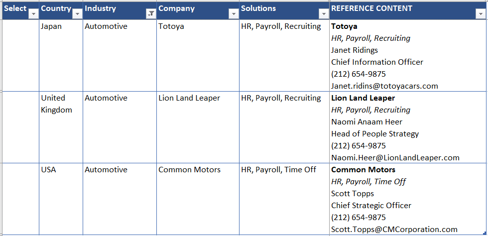
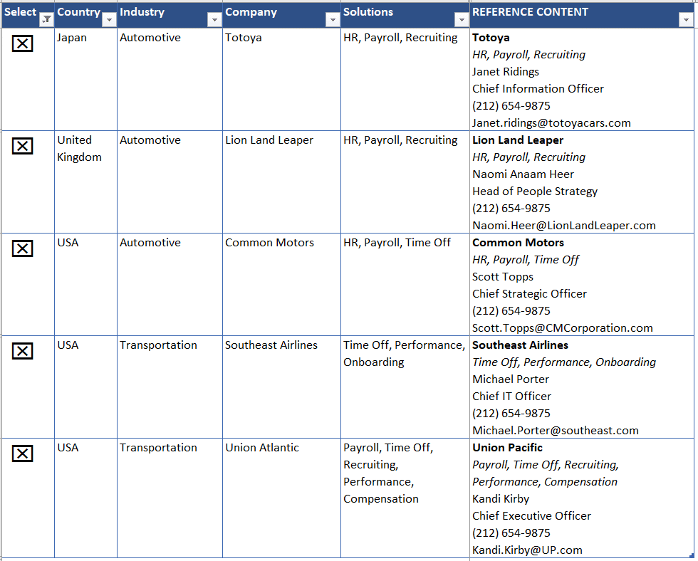
At the simplest level, you will want to create an Excel Spreadsheet with a row for every reference and a column for the reference content as well as for other important information and every criterion that you may want to use to guide the selection.  In this (made up) example each row contains a column for country, industry, implemented solutions, and the reference content itself.

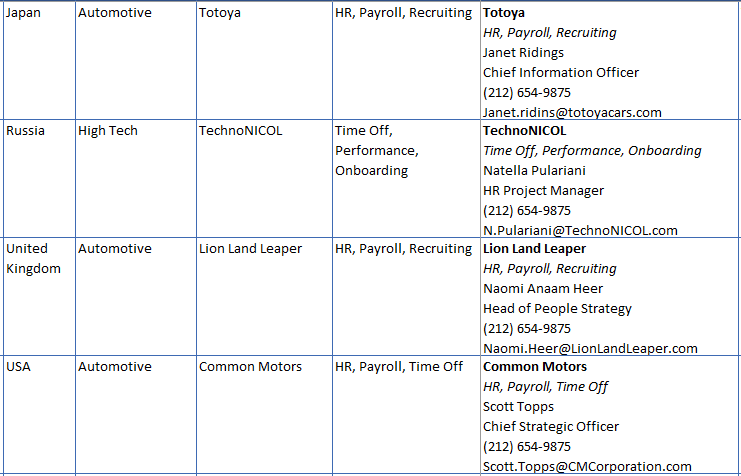
The number of columns you need will depend on the number of criteria that are relevant to your business.  Remember, you will want to add criteria that may be relevant, even if they are not always so.

The task of gathering all this data may seem daunting.  You may not have even ever fully considered the types of criteria that could be relevant.  But don’t be deterred.  Start with a few columns that are easy to establish and add columns as you evolve the process.

Excel Tables

After you have assembled your data into the appropriate rows and columns on your spreadsheet, it is time to apply a little Excel magic.

To the References spreadsheet, we want to first add one additional column that will help us keep track of our reference selections.  Select column ‘A’, right click and select ‘Insert’ from the popup menu.  If you haven’t already done so, add a row at the top and enter headings for each column:

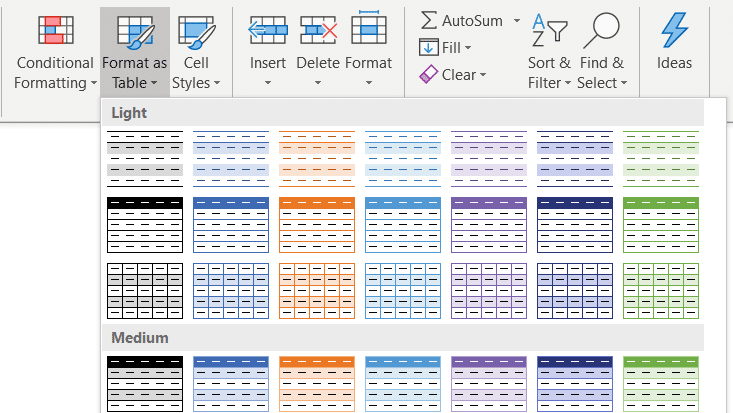
Select all the rows and columns that contain content. (Be sure to include the heading row.)  Go to the Excel ‘Home’ tag.  Toward the center of the ribbon, you will find a ‘Styles’ group.  Click on the ‘Format as Table’ dropdown.  Select a style that you like.

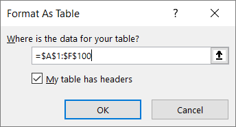
You will be prompted to confirm the range for the table. Nothing to do here if you have selected all the correct rows and tables. But be sure to check ‘My table has headers.’

Fun with Filters

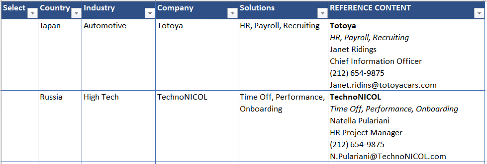
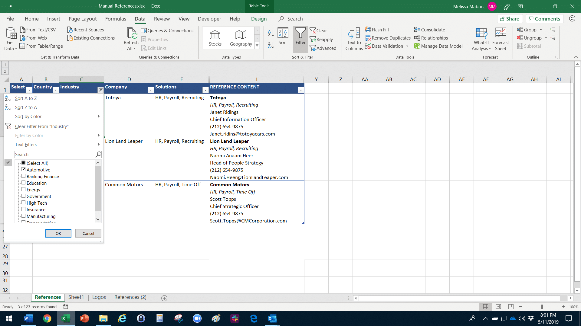
The advantage of turning your spreadsheet into a table, besides looking very nice, is that some very cool features are automatically applied. One you will notice right away is the appearance of filters on all the columns.  These appear as small down arrows in the heading row:

When you click on a filter button you can see a list of all the values for that column.  Uncheck ‘All’ to clear the selection and click on the value that you want to use as a criterion.  In our example, we are selling to an automotive manufacturer, so we will start by selecting ‘Automotive’ to see what references match that industry:

Three references have ‘Automotive’ entered as their industry.  Only these three rows are shown.  All the other rows are hidden.

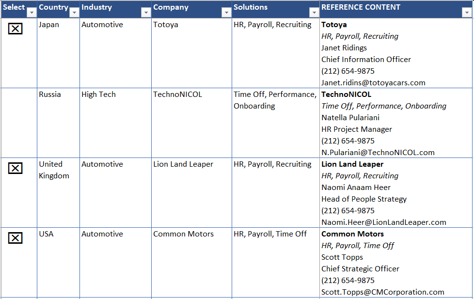
However, five references are required by the RFP.  I will need to expand my criteria.  But how will I keep track of these three that I have already found?  This is where our helper ‘Select’ column comes into play.  Type an ‘x’ in the ‘Select’ column of each row.  Then clear the filter you just applied.  To clear a filter, go back to the dropdown and select ‘All’ or click the small ‘Clear’ button on the ‘Data’ tab. (More about that later.)  All the rows will appear but the ‘selected’ rows will have an ‘X’ in the Select column.  (To get the checkbox appearance, format the column with ‘Windings’ font.)

To identify the other two, I can use the same process of narrowing down the list by selecting a different filter, typing ‘x’ in the ‘Select’ column, and clearing the filter when I am done.  When I have made my final two selections, I then use the ‘Select’ column filter to select just the rows with an ‘x’.

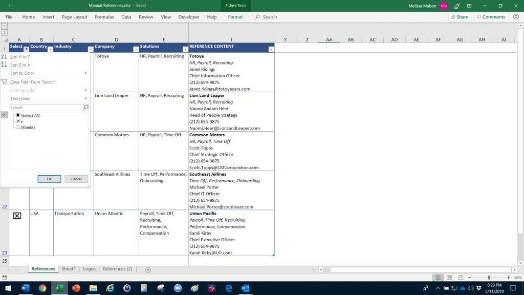
This will produce a table showing only the five selected rows that I have identified as the best references for this proposal.

Adding the Selected References to the Proposal

In our References table, the actual reference content is stored as a cell value in each row.  Although Excel is much more limited in formatting capabilities than Microsoft Word, it does support some basic direct formatting inside a cell.  In this case, we are using bold and italics in the reference content.

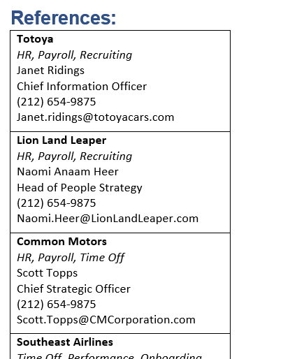
If the content sufficiently simple and is formatted properly in Excel, bringing the references into the final Word proposal is as simple as copying the reference content column and pasting it into the Word document.

When pasting the content into Word you have several choices. You can select one of the paste options on the Ribbon.  Hover over the item to see how the table will appear. (You can also try the additional options in Paste Special.)

If you paste it in as a table (recommended), you can change the formatting as needed directly in Microsoft Word.

If the content of the references is too complex to be stored in a single cell in Excel, you can store a link or instruction to find the reference content to be used.

Tips & Shortcuts

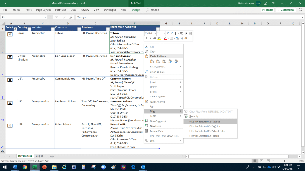
Apply filter on a single value: Place your cursor inside a cell with the value on which you want to filter. Click the ‘menu’ key if your keyboard has one (a little box with lines on the right between Alt and Ctrl). If it doesn’t, right click to show the popup menu.  Type ‘EV’ or click on ‘Filter by Selected Cell’s Value.’ The Filter will be applied without unchecking ‘All’ first. If you need to filter on MORE than one value, you will need to use the filter dropdown instead.

How Expedience Software Integrates with Excel References and Case Studies

Expedience Proposal Software custom Excel tools extend the functions of Microsoft Excel and Microsoft Word to generate targeted, beautifully formatted references and case studies.